KL Divergence: An Overview
I must admit that my first encounter with the so called Kullback-Leibler divergence was underwhelming. Whether it was the esoteric formula, or the fact that it was grouped together with what seemed like a dozen other entropy formulas; all I can say is that I didn’t like it.
Hiding behind that scary formula, however, KL divergence is a very useful and practical tool for evaluating data compression algorithms. In this post, I hope to explain and demonstrate the uses of this measure.
What is KL Divergence?
In a nutshell, KL divergence is a measure of how different two probability distributions are. The formal definition of KL divergence follows
\[D_{KL}(P||Q) = \sum_{x \in \chi} P(x) \log \frac{P(x)}{Q(x)}\]Where
- \(P(x)\), \(Q(x)\) are probability mass functions
- \(\chi\) is the set of possible \(x\) values
Observing the formula, a few conclusions can immediately be drawn. First of all, KL divergence is not a distance function, as it is not commutative. That is, \(D_{KL}(P||Q) \neq D_{KL}(Q||P)\). Perhaps a less obvious conlusion is that the KL divergence is always non-negative: \(D_{KL}(P||Q) \ge 0\). This result is not obvious, and is a result of the so called Gibbs’ inequality.
Why is KL Divergence?
Mathematical definitions are all well and good, but the previous section doesn’t demonstrate the real power of this measure. I will now present an alternate definition of KL divergence with respect to data compression.
If an information source follows a probability distribution \(P(x)\), and we were to model this information source using the distribution \(Q(x)\), the KL Divergence, \(D_{KL}(P||Q)\) represents the excess entropy that this model would produce.
Example 1 - Huffman Coding
Consider the following information source:
| Symbol | Prob |
|---|---|
| A | 0.9 |
| B | 0.07 |
| C | 0.03 |
Table 1: The information model
The entropy of this source is \(H(X)\approx 0.557\frac{\mathrm{bits}}{\mathrm{symbol}}\). This entropy represents the theoretical, most optimal way to represent the data. In order to efficiently code this information source, we will use a Huffman code. Below is the Huffman code table.
| Symbol | Code |
|---|---|
| A | 1 |
| B | 01 |
| C | 00 |
Table 2: Huffman codes for model
While the Huffman code is better than a naïve coding method, it is not the most optimal method for encoding this information source. We can calculate the average code length for this coding method and compare it to the optimal case.
\(\mathrm{Average\ Length}=(0.9)(1\,\mathrm{bit})+(0.07)(2\,\mathrm{bits})+(0.03)(2\,\mathrm{bits})\) \(=1.1\frac{\mathrm{bits}}{\mathrm{symbol}}\)
Comparing this to the information entropy, we see that our method uses \(0.543\) more bits per symbol than is optimal. We can say that the Huffman model produces \(0.543\) bits of excess information per symbol. How are we to understand this inefficiency?
Let’s forget about the actual underlying information model and focus on the Huffman table. I propose a question: if the Huffman table shown in Table 2 were optimal, could we infer the probability model that it represents? Well, symbols B and C have the same code length. If the Huffman model were optimal, that would imply that B and C occur with equal probability. Symbol A has half of the code length as B and C, and thus must occur with twice the probability of B and C. With these observations, we can construct the underlying, ideal probablility model of the Huffman table.
| Symbol | Code | Implied Probability |
|---|---|---|
| A | 1 | 0.5 |
| B | 01 | 0.25 |
| C | 00 | 0.25 |
Table 3: Huffman codes for model with implied probabilities
With this implied probability model, we now have all the pieces for calculating the KL divergence. Namely, we have \(P\), the information model, and \(Q\), the Huffman model we created to approximate \(P\). Calculating the KL divergence, we find that it is exactly equal to the excess information from the Huffman model:
| Symbol | P(x) | Q(x) |
|---|---|---|
| A | 0.9 | 0.5 |
| B | 0.07 | 0.25 |
| C | 0.03 | 0.25 |
With this result, we come to a fascinating result:
The efficiency of a coding method is a result of its probability model; specifically, how the model diverges from the underlying model.
This example illustrates how the KL divergence can be used to predict the performance of a probability model.
Example 2 - KL divergence as an optimization parameter
Consider an information source with 50 symbols. The probability model of the source is shown below: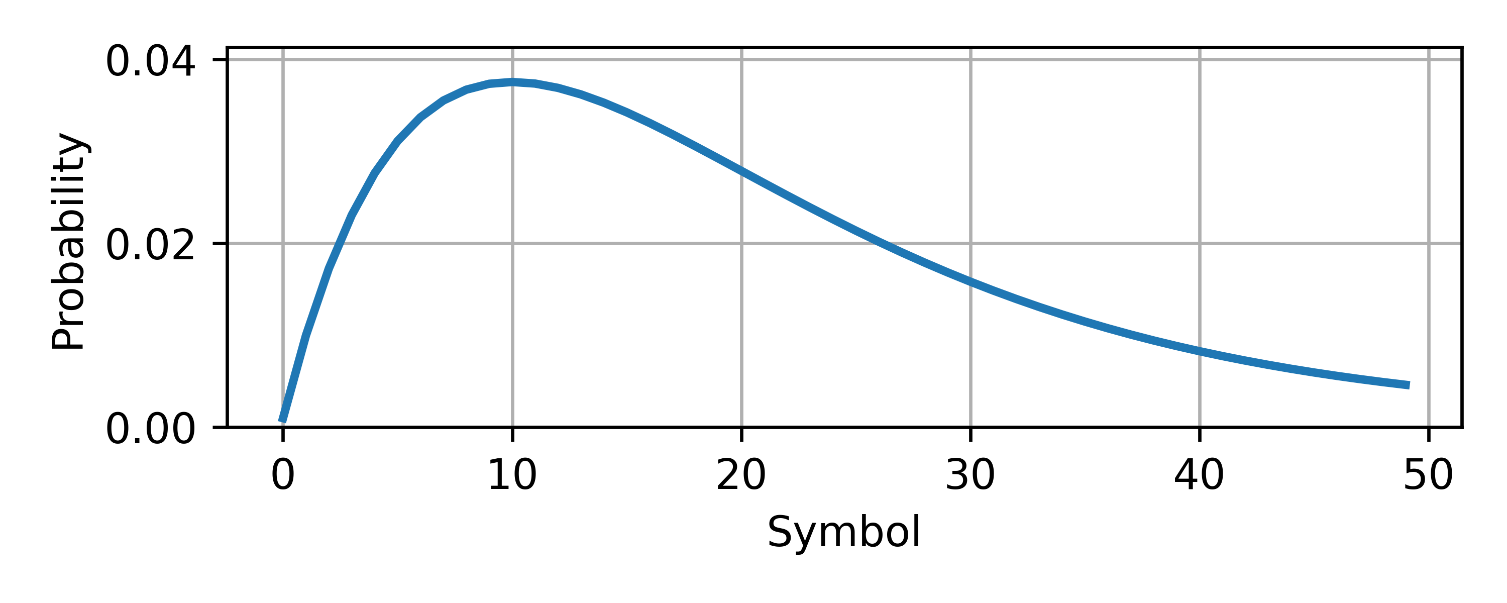 Assume that our algorithm allows us to model information in one of two ways:
as a uniform random variable or as an exponential random variable with a single parameter \(\lambda\)1. The questions we want to answer are
Assume that our algorithm allows us to model information in one of two ways:
as a uniform random variable or as an exponential random variable with a single parameter \(\lambda\)1. The questions we want to answer are
- Should we use a uniform random variable or an exponential?
- If we use an exponential random variable, what value of \(\lambda\) will produce the most optimal code?
We will now solve these problems.
2.1 - Calculating KL divergence in Python
The following code will be used to calculate the KL divergence between two probability models:
def kl(p,q):
    return sum(scipy.special.rel_entr(p,q))/np.log(2)
This function assumes properly formatted inputs and uses scipy’s rel_entr function. The scaling factor of \(\ln(2)\) converts the output from nats to bits.
2.2 - KL divergence optimization
We can use scipy’s optimization functions to find which value of \(\lambda\) will minimize the KL divergence of the model.
# Calculates an exponential distribution (truncated)
# with parameter 'l'
def exp(n,l):
    p = l * np.exp(-l*n)
    return p / sum(p)

# Find optimal exponential distribution
f = minimize_scalar(lambda x : kl(p,exp(n,x)))
l_optimal = f.x
l_divergence = f.fun
print("Exponential Divergence: {} using lambda = {}".format(l_divergence,l_optimal))

# Uniform distribution
p_uniform = np.ones(50) / 50.0
print("Uniform divergence: {}".format(kl(p,p_uniform)))
Running this script, we get:
Exponential Divergence: 0.1395 using lambda = 0.02978
Uniform divergence: 0.2666
We see that the exponential distribution is a better model, and the optimal value for \(\lambda\) is:
\[\lambda_{optimal}\approx0.02978\]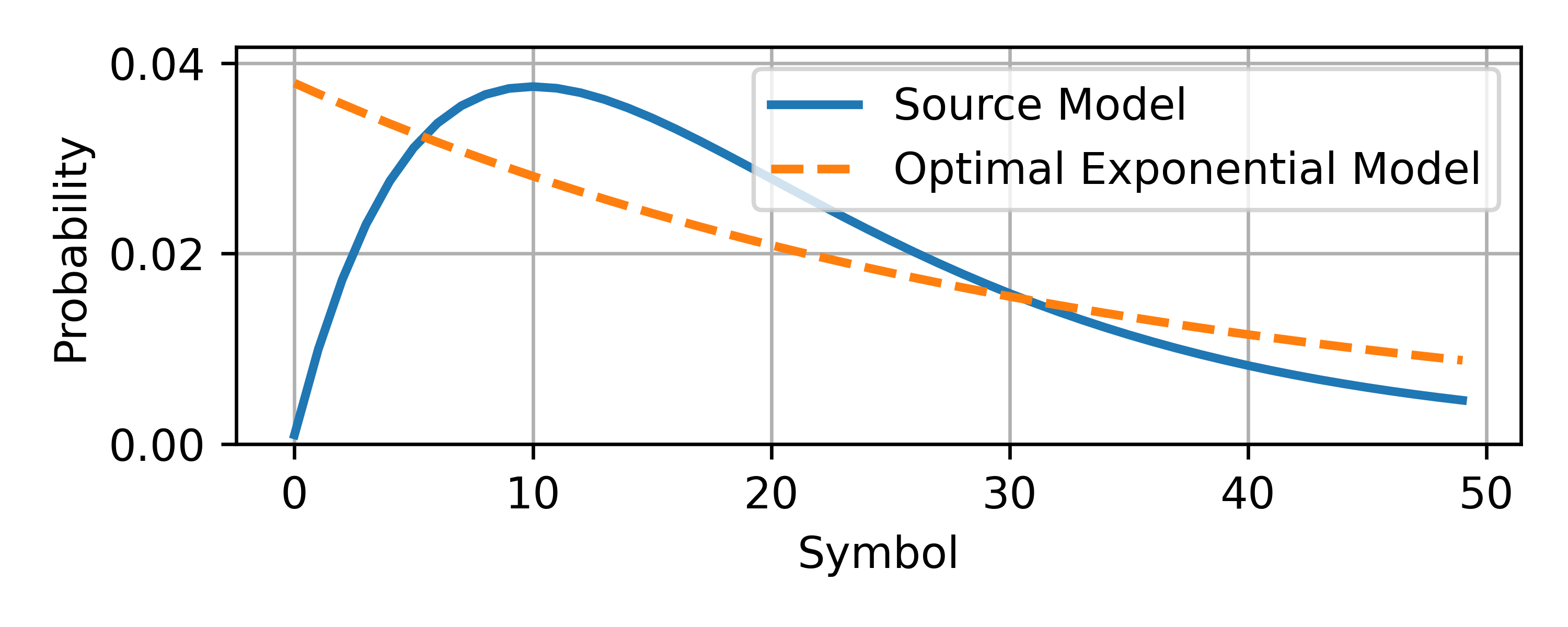
Notice from the graph above that, while optimal, the exponential model does not perfectly represent the information source. In fact, it appears to diverge from the information model toward the left side of the graph. If you were evaluating graphically, you might be temped to use a lower value of \(\lambda\) in order to close this gap. Ultimately, blindly chosing a probability model is difficult and unintuitive. KL divergence makes it easy.
Practical Considerations
By this point you understand that
- Using a proper probability model determines how effective your data compression will be.
- KL divergence is the tool to determine said model.
These points, however, beg the question: if the model is so important, what is the best probability model, and why don’t we just use that? Hopefully it’s obvious to you that the best probability model would be to use the exact model of the information (i.e. \(P=Q\)). It can be easily shown that \(D_{KL}(P||P) = 0\) excess bits.
Unfortunately, it’s not so easy.
Designing a sufficiently generalized compression algorithm means that you’ll be encountering a variety of information sources, each with it’s own probability model. In order to decompress the data, the decompressor must have knowledge of the probability model used to compress the data. What this means in practice is that you’ll have to store both the compressed data and the probability model used to compress it.
Let’s return to Example 2. Let’s say we had to encode 100 symbols from this information source. There are 50 different symbols and the information entropy is \(\approx 5.39\frac{\mathrm{bits}}{\mathrm{symbol}}\). It’s pretty easy to see that we would need on average \(\approx 539\,\mathrm{bits}\) to encode this stream.2 This size neglects the probability model, however. If we encoded the probability model as an array of 32-bit floating point numbers, the total size of the stream would then be:
\[(32)(100) + 539 = 3739\,\mathrm{bits}\]This comes out to \(37.39\) bits per symbol. Yikes! In this case it would be more efficient to store each value as a 32-bit integer.
Now lets consider using the exponential model described in Example 2. The optimal model has a KL divergence of \(0.1395 \frac{\mathrm{bits}}{\mathrm{symbol}}\). Because it’s a single parameter however, we can store the entire probability model using two numbers: \(\lambda\) and \(N_{\mathrm{symbols}}\). If we stored these using a 32-bit floating point and an 8-bit integer respectfully, we would end up with a total size of:
\[32 + 8 + (100\,\mathrm{symbols})(0.1395 + 5.39\,\frac{\mathrm{bits}}{\mathrm{symbol}})\approx 593\,\mathrm{bits}\]A serious improvement. Notice that the approximated model adds excess entropy per symbol to the total, but this is outweighed by the model’s small size. In general, the size of a compressed data set will be
\[N_{\mathrm{ProbabilityModel}} + \left[H(X) + D_{KL}(P||Q)\right]N_{\mathrm{symbols}}\]Where
- \(P(x)\) is the probability mass function of the information source
- \(Q(x)\) is the approximation of \(P(x)\)
- \(H(X)\) is the information entropy of the source
- \(D_{KL}(P||Q)\) is the KL divergence
- \(N_{\mathrm{symbols}}\) is the number of symbols to encode
- \(N_{\mathrm{ProbabilityModel}}\) is the number of bits used to store \(Q(x)\)
The theoretical limit of the size is \(H(X)N_{\mathrm{symbols}}\).
If we subtract this from the total size, we get the total excess information:
\[N_{\mathrm{ProbabilityModel}} + D_{KL}(P||Q)N_{\mathrm{symbols}}\]This illustrates the trade off between a high accuracy model and a low accuracy one. Indeed, if the number of symbols is sufficiently high enough, it may be more efficient to use a higher accuracy model. The following example illustrates this.
Example 3 - Real World Application
I have coded a function which produces symbols that match the information model in Example 2. Using constriction, we will test how different probability models can compress a stream. Below is the function that produces the symbols.
# PMF -> CDF
pc = np.cumsum(p)

def get_symbol():
    r = np.random.rand()
    for i in range(50):
        if pc[i] > r:
            return i
    return 49
We will create two models using constriction. Note that I use \(\lambda = 0.1\) rather than the ideal value.
information_model = constriction.stream.model.Categorical(p)
approximate_model = constriction.stream.model.Categorical(exp(n,0.1))
We will test these models at different stream sizes:
approximate_size = []
size = []

Ls = [int(x) for x in np.linspace(100,5000,100)]
for L in Ls:
    symbols = np.array([get_symbol() for _ in range(L)], dtype=np.int32)
    coder = constriction.stream.stack.AnsCoder()
    coder.encode_reverse(symbols, information_model)
    size.append(coder.num_bits() + 32*50)

    coder2 = constriction.stream.stack.AnsCoder()
    coder2.encode_reverse(symbols, approximate_model)
    approximate_size.append(coder2.num_bits() + 32 + 8)
Below we have the results.
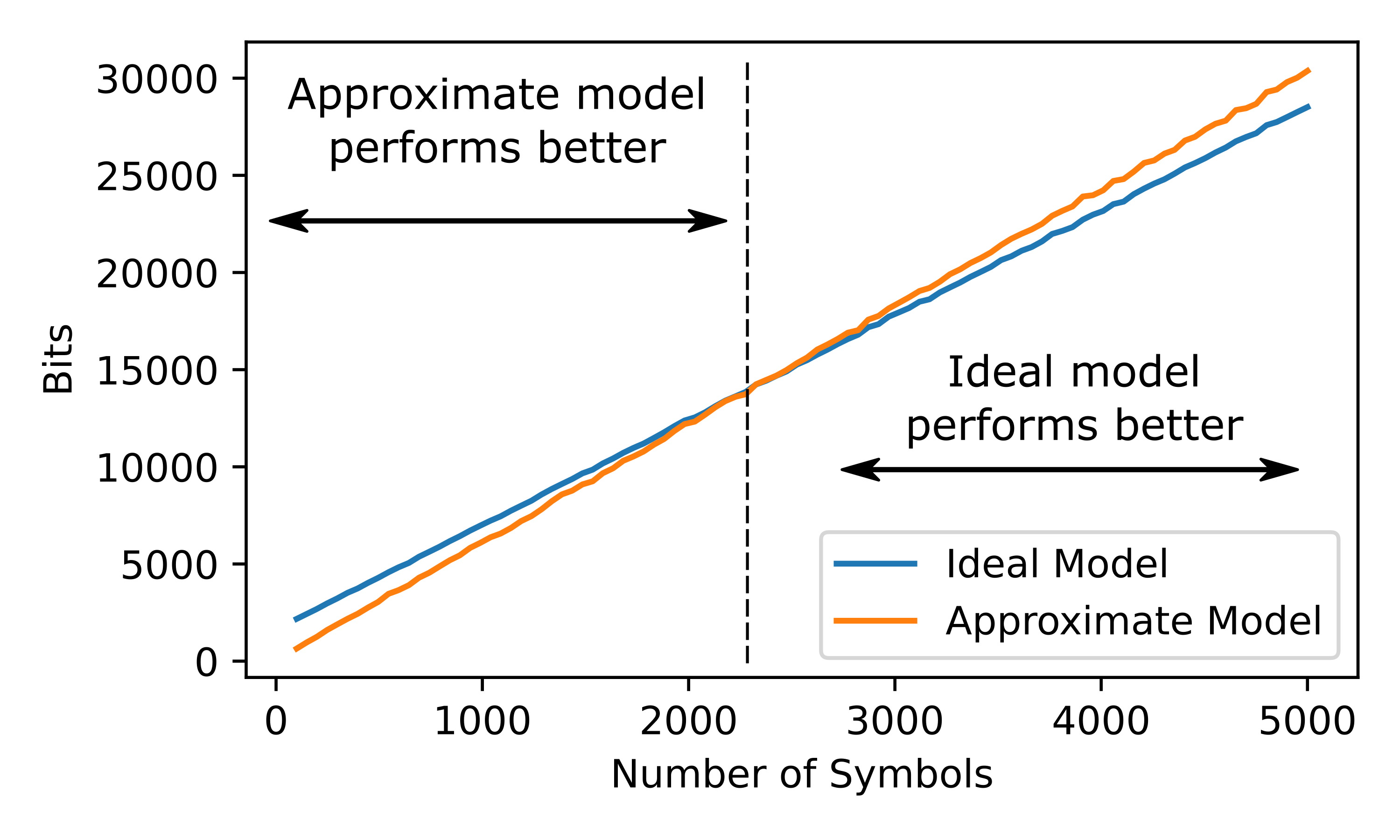
Notice that, for short streams, the approximate model performs better. This is due to the small size of the model compared to the ideal model. As the number of encoded symbols grows, we see that the ideal model begins to perform better.
Conclusion
I hope this article has illustrated both the theoretical and practical applications of KL divergence. Used properly, this measure is indepensable in the field of data compression.