Calculus on the Atchafalaya

The Department of Transportation and Development in the state of Louisiana has implemented a new safety measure for the Atchafalaya Basin Bridge. The new rule automatically issues speeding tickets to anyone caught speeding over the bridge. To enforce this rule, DOTD has setup an automated camera system that timestamps every vehicle as it enters and exits the bridge.
In the words of DOTD:
“if you cross the bridge in less than 18 minutes, you will get a ticket in the mail.”
The system seems fool proof: the bridge is 18 miles long, and the speed limit is 60 miles per hour. If you cross the bridge in under 18 minutes, you must have exceeded the speed limit.
But… is this true?
This question no doubt plagued the famous 19th century mathematician Augustin Louis Cauchy. A Frenchman himself, Cauchy no doubt had the Cajun people in mind when he formalized and proved the Mean Value Theorem.
In this article, I’ll introduce the mean value theorem and show how it can be applied to this problem. Along the way, I’ll touch on the basics of differential calculus; specifically, how we can relate bridges and speed limits to slopes and arcs.
Let’s begin with a brief introduction to the mean value theorem.
Mean Value Theorem
The mean value theorem states the following:
For any smooth planar arc between two endpoints, there is at least one point at which the tangent to the arc is parallel to the secant through its endpoints.
In this form, the theorem is entirely geometric. Before we apply this theorem to bridges and speed limits, let’s look at a few examples to refresh our minds. First off: what is a ‘smooth planar arc between two points’?

Like the figure above, an arc is basically any path that connects between two points. It’s really that simple. 1
The mean value theorem relates the tangents and secant of the arc. These words should be familiar to you if you’re a 10th grade student (or an ancient Greek philosopher). For the rest of us, let’s review.
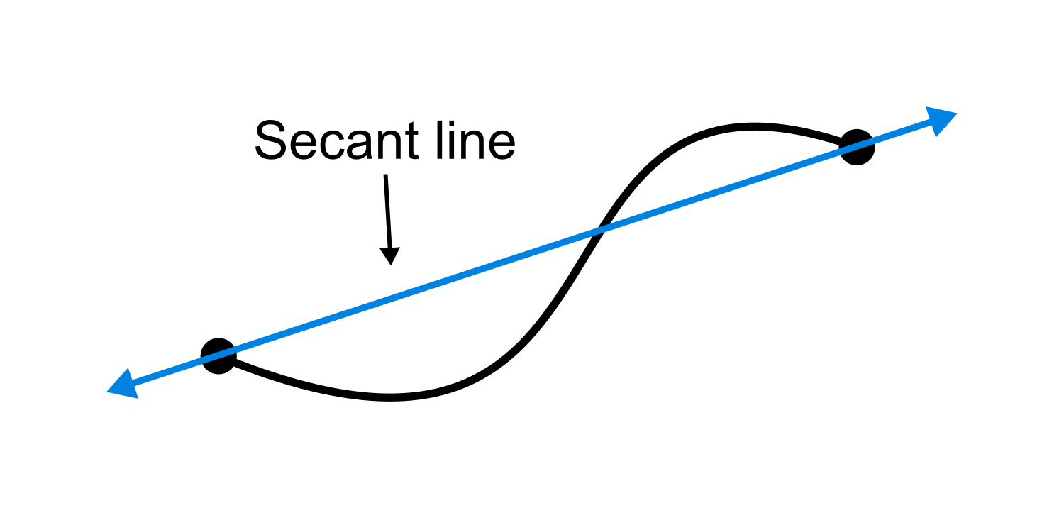
The secant of an arc is the line that passes between the two endpoints. The figure below shows the secant line in blue. An arc has only one secant line.
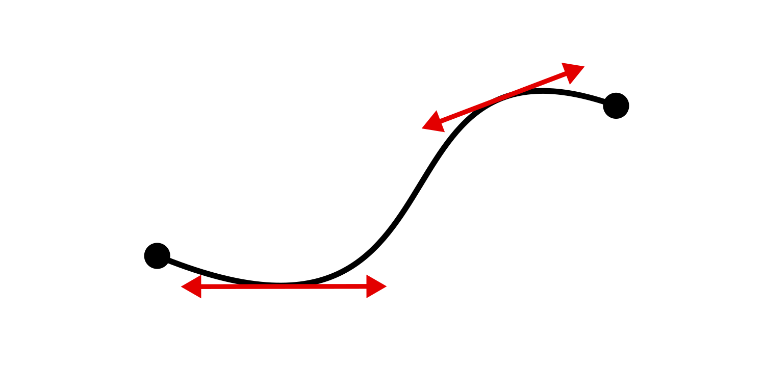
A tangent line is a line that just… barely touches the arc. If it was a bullet, you would say that it grazes the arc.2 The figure below shows a few tangent lines in red at points on the curve. Each point on a smooth arc has its own tangent line.
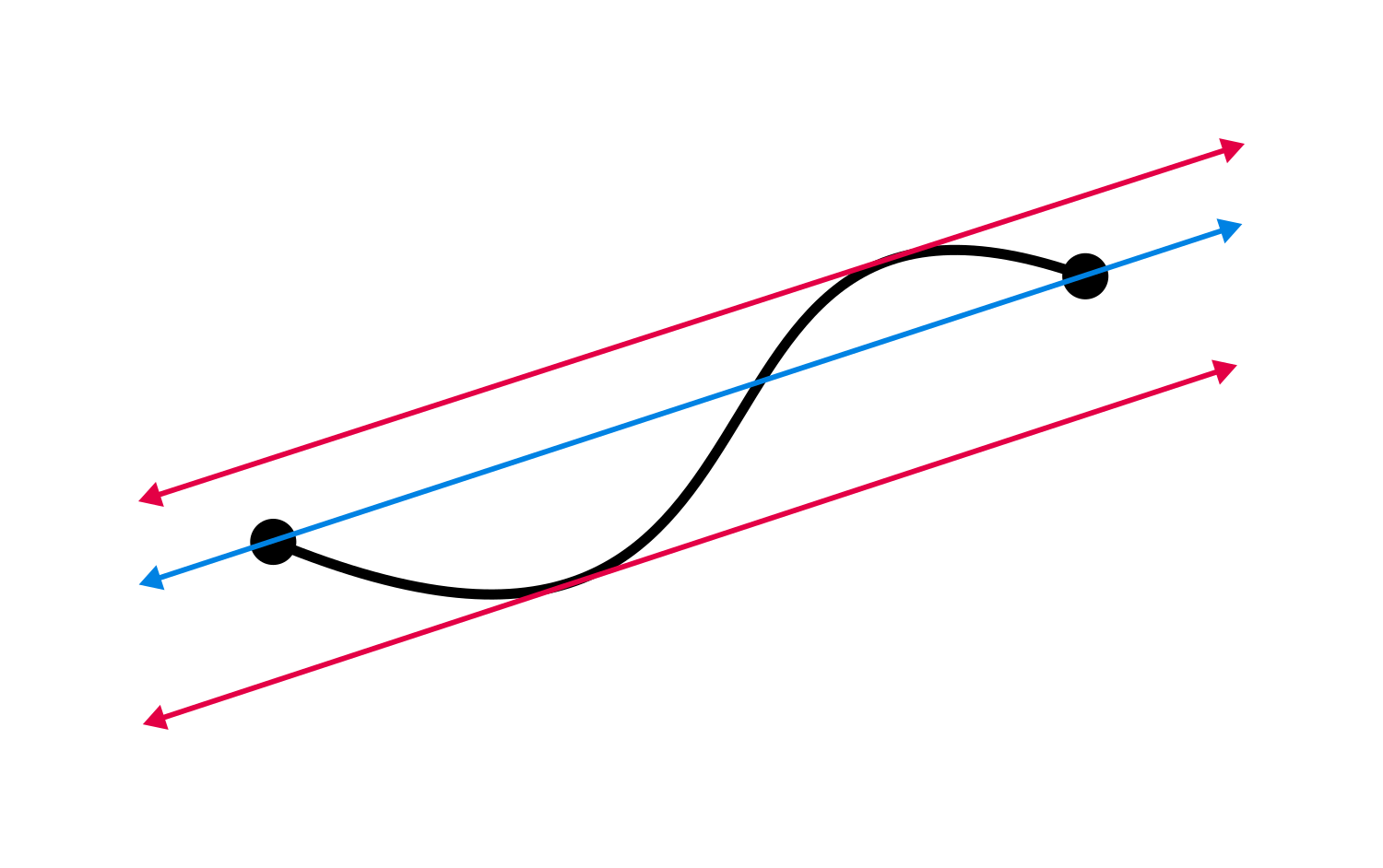
The mean value theorem states that there is at least one point on the curve where the tangent line is parallel to the secant line. On the curve above, there are actually two points where the tangent is parallel. The figure below shows this.
That is, in a nutshell, the idea of the mean value theorem.
But what’s all this got to do with speed limits?
Speed and Geometry
If we want to apply the mean value theorem to this problem, we need to relate speed to geometry in some way. Suppose you’re driving across the bridge at a constant rate of 54 miles per hour. At that rate, the trip across the 18-mile bridge will be exactly 20 minutes long. We can represent your trip visually using a graph:
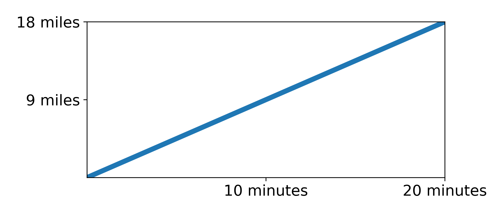
On this graph the horizontal axis represents time and the vertical axis represents distance. The blue line represents your trip. By itself, there’s not too much interesting going on here.
Now suppose that you double your speed: 108 miles per hour. For this trip, it only takes 10 minutes to cross the bridge. The graph looks different too:
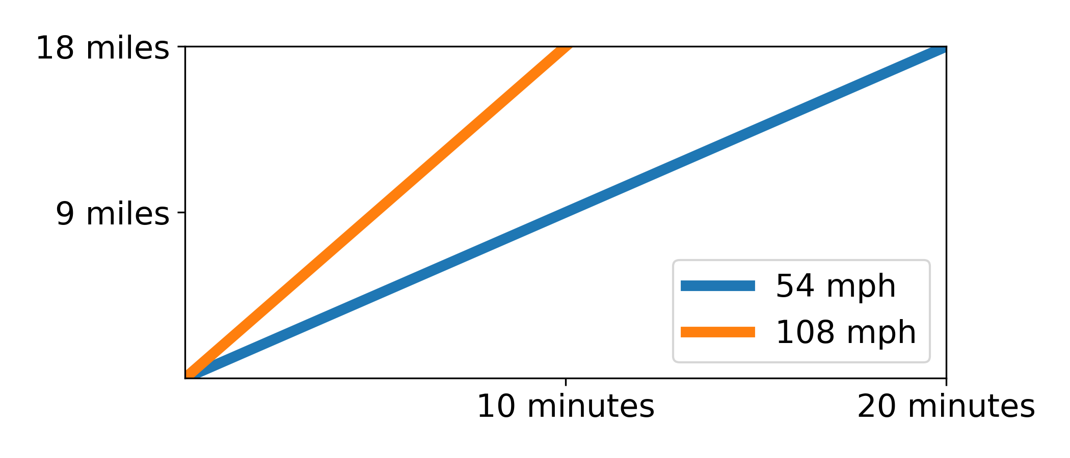
The graphs for both trips form a line on the plot. The difference between these two lines? Their slope!
The orange line, representing the 108-mph trip, has twice the slope of the blue line.
If you remember your algebra, you should know the formula for the slope of a line: “rise over run”, or, \(\frac{\Delta y}{\Delta x}\).
Let’s calculate the slope of the blue line. Remember that the horizontal (\(x\)) axis represents time in minutes and the vertical axis (\(y\)) represents distance in miles.
\[\mathrm{Slope} = \frac{\Delta y}{\Delta x} = \frac{18\,\mathrm{miles}}{20\,\mathrm{minutes}}\] \[=54\,\mathrm{mph}\]That’s right: the slopes of the line on the graph are actually the speed of the vehicle.
This is a very important result. The slope of a line is a geometric property. By using the distance-time graph, we can relate the speed of the vehicle to the slope of a line. This allows us to geometrically analyze a vehicle’s speed.
There’s only one problem.
If you’ve ever driven across the basin bridge, you’ll know that achieving a ‘constant speed’ is… unlikely. Traffic jams, accidents, couillons on the road… All these factors will cause slowdowns and speedups along your route. By the time you reach the end of the bridge, your distance graph will likely look something like this:
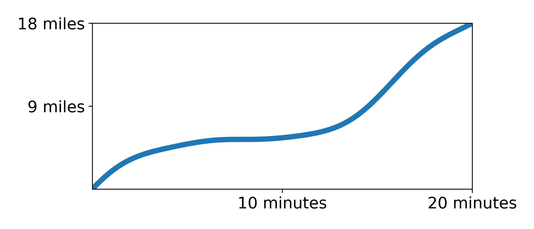
Which is to say: not a line. This throws a bit of a wrench into our analysis. Because the graph isn’t a line, it has no slope. If the graph has no slope, we can’t measure its speed geometrically. If we can’t apply geometry to this problem, we can’t use the mean value theorem…
Tangents and Secants
Rather than giving up, let’s just try the next best thing. We’ll construct a line between the beginning and end of the graph.
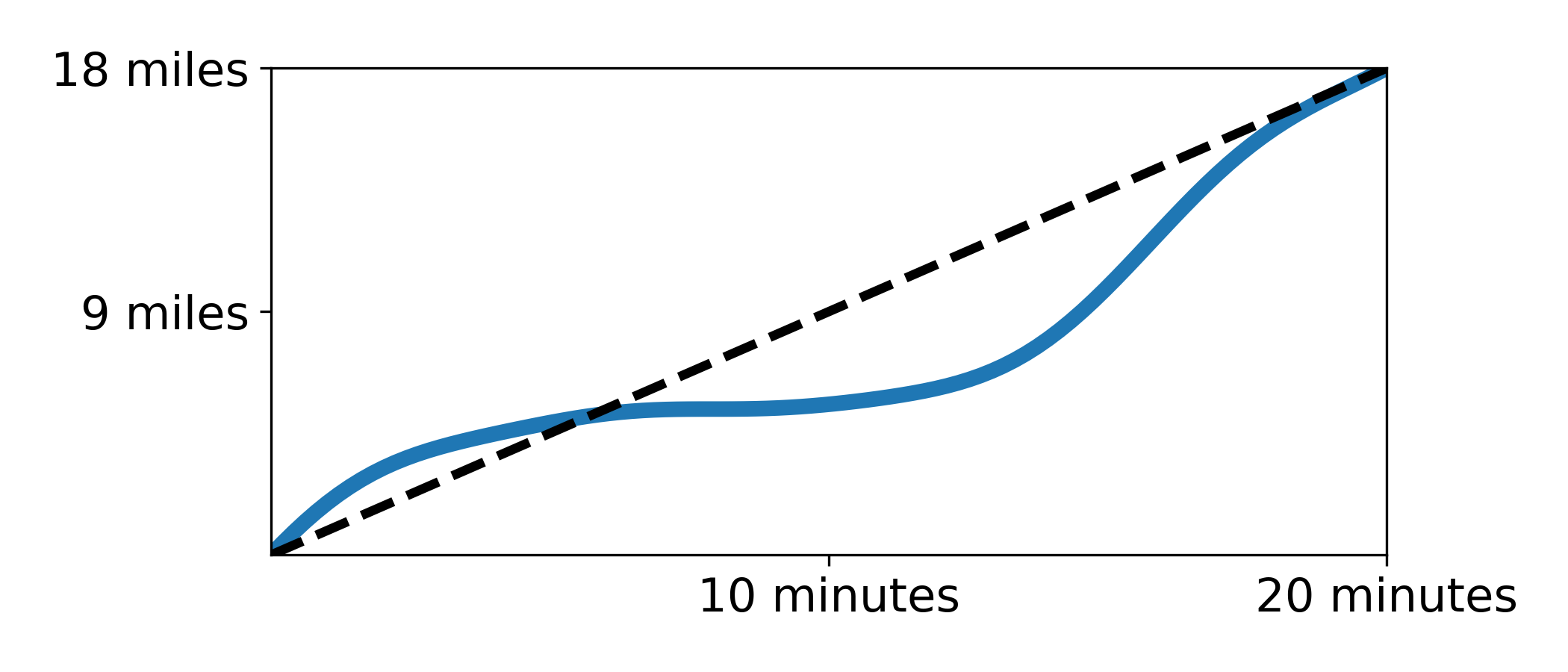
If we imagine this graph as an arc, this line is the secant. Because it’s a line, we can calculate its slope just like before. In this case we get the same result:
\[\mathrm{Slope} = \frac{18\,\mathrm{miles}}{20\,\mathrm{minutes}}=54\,\mathrm{mph}\]But remember, in this example, the vehicle’s speed is constantly changing. This slope doesn’t represent the speed per se; it represents the vehicle’s average speed. This is a very important result:
The slope of the secant line on the distance-time graph represents the average speed of the vehicle.
No matter how curvy or disjointed the graph gets, we can always get the vehicle’s average speed by constructing a secant line. Cool!
Remember that the mean value theorem relates secant lines and tangent lines. The obvious next question: what would a tangent line represent in such a graph?
Congratulations! You’ve stumbled into the field of differential calculus. The fathers of this field, Newton and Leibniz, tell us that the slope of a tangent line at a point represents the so-called instantaneous rate of change. In our case it represents the instantaneous speed. We can use a tangent line to measure the speed of the vehicle anywhere on the graph.
Amazing!
Before we get back to the mean value theorem, let’s review the results we’ve found thus far.
- If your speed is constant, the graph is a straight line. The slope of this line represents your speed.
- For any graph, we can calculate the average speed by measuring the slope of the secant line through the graph.
- We can measure the speed at any point on the graph by measuring the slope of a line tangent to that point on the graph.
Applying the Mean Value Theorem
Remember the original theorem:
For any smooth planar arc between two endpoints, there is at least one point at which the tangent to the arc is parallel to the secant through its endpoints.
We now have a clear connection between secants, tangents, and speed. We can rewrite the theorem to apply to our example:
For any trip across the bridge, there is at least one point at which your speed is equal to the average speed of the trip.
Let’s try an example. Imagine you drove across the bridge in 16 minutes. The graph below shows your position on the bridge over the 16 minute period.

Driving 18 miles in 16 minutes works out to an average speed of approximately 68 mph. As we discovered above, 68 mph is also the slope of the black secant line. More importantly, it is above the speed limit. According to the mean value theorem, there is at least one point on our trip where we are driving exactly 68 mph. The animation below shows the speed along the drive.
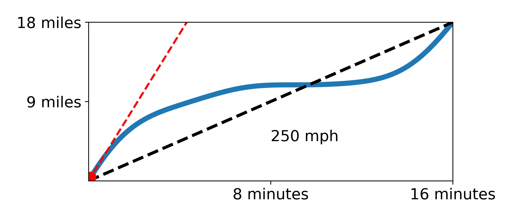
As we can see, there are in fact two different points at which the car is driving 68 mph. Notice how, at these points, the red tangent line is parallel to the secant line. This is exactly what the mean value theorem says!
For the two camera system implemented by the DOTD, calculating a vehicle’s average speed is relatively simple:
\[\mathrm{Avg.\,Speed} = \frac{18\,\mathrm{miles}}{\mathrm{Transit\,Time}}\]If the transit time is less than 18 minutes, then the average speed of your vehicle is greater than 60 mph. According to the mean value theorem, if your average speed exceeds 60 mph, you must have traveled greater than 60 mph at some point on your trip.
Busted! 3
The mean value theorem proves that you were speeding, even though the cameras never caught you doing it.
Conclusion
The result of this post may be underwhelming. You may even be tempted to say that the results are… obvious.
“Obviously, if my average speed was over the speed limit, then I was driving over the speed limit.”
There is, of course, a big difference between intuiting and answer and proving it. It takes quite an imagination to use a theorem about arcs, secants, and tangents and apply it to roads, bridges, and speed limits. It is that imagination that makes calculus so interesting.
Drive safe!
Notes
-
I left off the idea of a ‘smooth’ arc. The idea of smoothness is pretty intuitive, but does require a little bit of calculus to formalize. ↩
-
Students of geometry may be under the false impression that a tangent line is a line that only touches ‘at one point’. This is not the most general definition, and is actually wrong more often than not. It is correct in the context of a circle. ↩
-
Cauchy would probably have said: quod erat demonstrandum ↩